
Файл:Butterworth response.png
Арыгінальны файл (1240 × 880 піксэляў, памер файла: 86 кб, тып MIME: image/png)
|
|
Гэты файл паходзіць зь Вікісховішча. Зьвесткі пра гэты файл зь яго старонкі апісаньня прыведзеныя ніжэй. Вікісховішча — сховішча вольных мэдыяфайлаў. Вы можаце дапамагчы. |
Апісаньне
| Апісаньне |
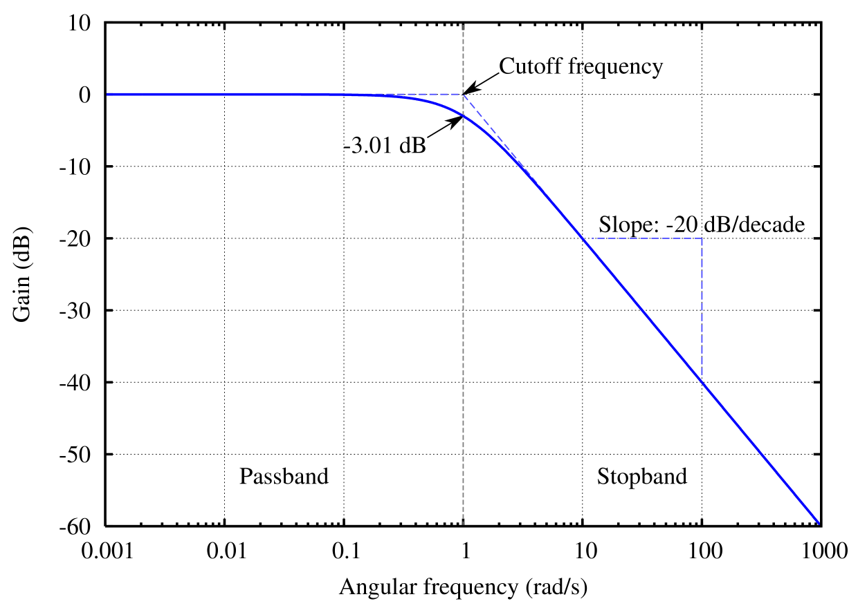
English: The frequency response of a Butterworth filter with logarithmic axes (Bode plot) and various labels. Cutoff frequency is normalized to 1 rad/s. Gain is normalized to 0 dB in the passband.
Many orders on one plot: File:Butterworth orders.png. Version with no text available at File:Butterworth plain.png, though you should probably just modify the source code and regenerate it in your own language. See Wikipedia graph-making tips. Generated in gnuplot with the script below (save as butterworth.plt and then open in gnuplot). Then I opened the butterworth.ps file in a text editor to edit the line colors and linestyles, as per this description. This avoids needing to open in proprietary software, and really isn't that difficult (especially if you don't know the commands in the proprietary software either). ;-) Identify the lines easily by their color (the arrow is currently magenta and I want it to be black. Ah, there is the entry with 1 0 1, red + blue = magenta) or by using the gnuplot linestyle−1. (For instance, gnuplot's linestyle 3 corresponds to the ps file's /LT2.) Then you can edit the colors and dashes by hand. I changed the original: /LT0 { PL [] 1 0 0 DL } def
/LT1 { PL [4 dl 2 dl] 0 1 0 DL } def
/LT2 { PL [2 dl 3 dl] 0 0 1 DL } def
/LT3 { PL [1 dl 1.5 dl] 1 0 1 DL } def
into this: /LT0 { PL [] 0 0 1 DL } def
/LT1 { PL [4 dl 2 dl] 0.5 0.5 0.5 DL } def
/LT2 { PL [6 dl 3 dl] 0.3 0.3 1 DL } def
/LT3 { PL [] 0 0 0 DL } def
/LT4–/LT8 I left unchanged. (I don't know what they're used for anyway.) /LTw, /LTb, and /LTa are for the grid lines and such.To convert the PostScript file to PNG:
|
| Дата | 26 чэрвеня 2005 (дата загрузкі) |
| Крыніца | Уласны твор |
| Аўтар | Omegatron |
| Іншыя вэрсіі |
|
| gnuplot source | click to expand
set samples 2001
set terminal postscript enhanced landscape color lw 2 "Times-Roman" 20
set output "butterworth.ps"

# Butterworth amplitude response and decibel calculation.  n is the order, which is just 1 in this image.
G(w,n) = 1 / (sqrt(1 + w**(2*n)))
dB(x) = 20 * log10(abs(x))

# Gridlines
set grid

# Set x axis to logarithmic scale
set logscale x 10

# Set range of x and y axes
set xrange [0.001:1000]
set yrange [-60:10]

# Create x-axis tic marks once per decade (every multiple of 10)
set xtics 10

# Use 10 x-axis minor divisions per major division
set mxtics 10

# Axis labels
set xlabel "Angular frequency (rad/s)"
set ylabel "Gain (dB)"

# No need for a key
set nokey #0.1,-25

# Frequency response's line plotting style
set style line 1 lt 1 lw 2

# Draw a separator between passband and stopband and label them
set style line 2 lt 2 lw 1
set style arrow 2 nohead ls 2
set arrow 3 from 1,-60 to 1,10 as 2

# Label coordinates are relative to the graph window, not to the function, centered at the 1/4 and 3/4 width points
set label 1 "Passband" at graph 0.25, graph 0.1 c
set label 2 "Stopband" at graph 0.75, graph 0.1 c

# Asymptote lines and slope lines are the same "arrow" style
set style line 3 lt 3 lw 1
set style arrow 3 nohead ls 3

# Draw asymptote lines
set arrow 1 from 1,0 to 1000,-60 as 3
set arrow 2 from .001,0 to 1,0 as 3

# -3 dB arrow style and arrow
set style line 4 lt 4 lw 1
set style arrow 4 head filled size screen 0.02,15,45 ls 4
set arrow 4 from 2,3 to 1,0 as 4

# "Cutoff frequency" label uses same coordinates as the function
set label 3 "Cutoff frequency" at 2,4 l

# "-3 dB" label
set arrow 5 from 0.5,-6 to 1,-3 as 4
set label 4 "-3.01 dB" at 0.5,-7 r

# Draw slope lines and label
set arrow 6 from 100,-20 to 12,-20 as 3
set arrow 7 from 100,-20 to 100,-39 as 3
set label 5 "Slope: -20 dB/decade" at 100,-18 c

# Plot the filter response
plot \
     dB(G(x,1)) ls 1  title "1st-order response"
|


|
Існуе вэктарная вэрсія гэтай выявы (SVG). Рэкамэндуецца выкарыстаньне вэктарнай выявы замест растэрнай.
File:Butterworth response.png → File:Butterworth response.svg
Болей інфармацыі пра вэктарную графіку чытайце ў дапамозе. |
 |
Ліцэнзія
- Вы можаце свабодна:
- дзяліцца – капіяваць, распаўсюджваць і перадаваць гэты твор
- ствараць вытворныя творы – адаптаваць твор
- Пры выкананьні наступных умоваў:
- пазначэньне аўтарства – Вы мусіце пазначыць аўтарства, падаць спасылку на ліцэнзію і пазначыць, ці былі зробленыя зьмены. Вы можаце зрабіць гэта любым разумным спосабам, але не такім чынам, каб склалася ўражаньне, што ліцэнзіят падтрымлівае вас ці выкарыстаньне вамі гэтага твору.
- распаўсюджваць на тых жа ўмовах – Калі вы зьмяняеце, трансфармуеце ці грунтуецеся на гэтым матэрыяле, вы мусіце распаўсюджваць ваш унёсак паводле той жа ці сумяшчальнай ліцэнзіі, што і арыгінал.

|
Дазвол на капіраваньне, распаўсюджаньне і/альбо зьмену гэтага дакумэнту згодна з умовамі GNU Free Documentation License вэрсіі 1.2 альбо больш позьняй, апублікаванай Фундацыяй вольнага праграмнага забесьпячэньня; безь нязьменных сэкцыяў і тэкстаў на першай і адвартонай вокладках. Копія ліцэнзіі ўключаная ў сэкцыю з назвай GNU Free Documentation License. |
Гісторыя файла
Націсьніце на дату/час, каб паглядзець, як тады выглядаў файл.
| Дата і час | Мініятура | Памеры | Удзельнік | Камэнтар | |
|---|---|---|---|---|---|
| цяперашняя | 20:45, 23 ліпеня 2005 | | 1240 × 880 (86 кб) | Omegatron | split the cutoff frequency markers |
| 19:31, 23 ліпеня 2005 |  | 1250 × 880 (92 кб) | Omegatron | Better butterworth filter response curve | |
| 22:54, 26 чэрвеня 2005 |  | 250 × 220 (2 кб) | Omegatron | A graph or diagram made by User:Omegatron. (Uploaded with Wikimedia Commons.) Source: Created by User:Omegatron {{GFDL}}{{cc-by-sa-2.0}} Category:Diagrams\ |
Выкарыстаньне файла
Наступная старонка выкарыстоўвае гэты файл:
Глябальнае выкарыстаньне файла
Гэты файл выкарыстоўваецца ў наступных вікі:
- Выкарыстаньне ў de.wikipedia.org
- Выкарыстаньне ў eo.wikipedia.org
- Выкарыстаньне ў et.wikipedia.org
- Выкарыстаньне ў fr.wikipedia.org
- Выкарыстаньне ў hi.wikipedia.org
- Выкарыстаньне ў it.wikipedia.org
- Выкарыстаньне ў ja.wikipedia.org
- Выкарыстаньне ў pl.wikipedia.org
- Выкарыстаньне ў pt.wikipedia.org
- Выкарыстаньне ў zh.wikipedia.org